Specifically, you could write patterns that track the flow of data through a program, and flag places they might “taint” in that flow, such as tracking user input flowing into an arbitrary eval function, like in the above example.
This first pass of taint analysis was only intra-procedural, meaning that within a file we could usually detect how the data flows. If the user input flowed into some function that was defined in another file though, and that other function had an eval, we wouldn’t detect it. This is called interfile analysis, for obvious reasons.
Many users had been asking for exactly this, and so two years later, in February 2023, we released the pro engine, the first version of Semgrep capable of tracking data flows across files.
Here's roughly how that interfile analysis worked. First, we'd take the source code and build a naming environment: a mapping that tells us the function foo called in file1 is the same foo defined in file2. With that in place, we'd compute the taint configs for the rule. Every Semgrep rule defines matching patterns for four categories: sources (user-controlled input), propagators (patterns that carry taint forward, like certain library calls), sanitizers (patterns that mark data as safe), and sinks (dangerous locations we flag if tainted data reaches them, such as eval). A taint config is the set of all those pattern matches found in the actual source code. From there, we'd run dataflow algorithms over each match—checking whether sources could reach sinks, and using the naming environment to follow data flow across file boundaries. The output is a set of taint signatures: a compact encoding of which sources could potentially reach which sinks.
At this point, if you’ve done any sort of static analysis you would think “and now you just need to check if the sources properly satisfy some conditions on the sink and you’re done.” Instead, to avoid having to move some of our more specific intrafile dataflow code to this new interfile approach and validate that the outputs are the same, we dropped the taint configs, and passed the signatures as an environment to the existing intrafile code. We then proceeded to, yes, recompute the taint configs, and then revisit all the functions, do a heck of a lot more dataflow analysis, and then finally do our condition checks. We called this approach “run taint twice.” There were some practical reasons we did this, which we’ll get into in the next section. In hindsight, Iago Aba,l who wrote the first pass of intrafile taint analysis, said at one point “if we had only taken a few more weeks, we could have just run taint once.”
Does it matter? Measuring the Performance Impact
Three years worth of building on top of that code later, in 2026, we have many more users of Semgrep, and performance just wasn’t cutting it (have you seen RAM prices recently???). So performance became a top priority, and us engineers were very excited about it. Our minds turned to Brandon Gregg’s performance and benchmarking mantras, specifically “Does it matter?” and “Do it, but don't do it again”.
Of course we can’t avoid doing taint analysis, but did we have to do it twice? But also, there were three years worth of code built on top of this, and it’s not trivial to make major changes to an algorithm like this without risking slight differences that significantly increase the noise of the security issues Semgrep finds. If a user wakes up tomorrow and sees that a SQL injection is no longer there, even though they didn’t fix it, they will be far less trusting of us, even if Semgrep runs 2x faster. So although it’s obvious that running taint once would be a performance boost, we needed hard numbers, or risked getting egg on our faces because we “swore” this is the slow part (even though it almost certainly was) and then a quarter of work later nothing got faster.
As mentioned in the last blog post, we have a handy dandy new profiler, and a whole suite of other observability tools to confirm this. Peaking at the profiles from that time, we see we do in fact spend a significant amount of CPU time in the relevant taint functions, specifically, for a period of 53 days worth of cpu time, we spend ~18 days on our first taint pass, and ~7 days on the second.
It’s important to remember that this is a measure of CPU time, NOT wall clock time. So if we spend 10 minutes across 6 cores, that’s one hour of cpu time. We can see at the top of the callstack for the second taint pass, Stdlib__Domain.spawn.body, which is the function called by multithreaded code, so we know that’s parallel, but the first pass isn’t a child, so we know that is indeed wall clock time. Another important note here is that this is the sum of all profiles across 1% of scans, so if 100 scans complete in 1 minute, and one scan spends 24 hours in taint analysis, that could also cause this sort of graph. At this point, the CPU cost alone justifies the effort: the first pass of taint accounts for roughly a third of total CPU time — and it isn't even parallelizable. We can't just throw more cores at the problem.
Worst case scenario here we save some major cloud costs, and if we’re smart we can lower perceived wall clock time by enabling parallelization of a huge chunk of code. I did end up adding tracing to the relevant functions later in the project, and that data confirmed our hypothesis. , It was time to run taint just once.
Implementation: How We Redesigned Taint Analysis to Run Once
Unlocking Parallelization with OCaml Multicore
As mentioned earlier, there were some practical reasons we didn’t implement this project earlier. The primary reason was that before OCaml 5.0 was released, there wasn’t a fantastic parallelism story. There’s a great talk here that was given at Fun OCaml by my peers Nathan Taylor and Nat Mote that dives deeper into this, so I’ll keep it short. Pre 5.0, we had to fork the process to achieve parallelism, which resulted in increased memory usage by a factor of up to the number of processes we created. This was barely tolerable for intrafile, since we could get away with only keeping a handful of taint configs and files in memory at one time, since we were only ever doing work on the context of one file.
If we were to run taint once though, we’d want to combine the dataflow passes and taint config generation of the two passes, which ultimately meant we would have to keep a whole bunch of taint configs and parsed source in memory all at once, or at the very least swallow the cost of serializing data to disk. This would not scale with this parallelism approach, as the first pass of taint already was pushing it memory wise. Now that we have multicore, running taint once became practical.
Death by a Thousand Tests
The first pass of running taint once was actually somewhat “simple,” in the sense that it was more or less a refactoring, and we had already attempted this before. Once the code was laid out before us, we could run our tests to see what broke. We quickly saw over 200 tests were failing, so we started splitting them up by language, to determine what specific part of the dataflow steps were relevant. For example, one step is to check dataflow from top level statements in Python, to actual function calls, as not all languages have top level statements. This was part of the second taint pass, but not the first, so we needed to move it over, and slot it in nicely to keep the code maintainable. None of these failing tests were especially surprising, we just had to work through them all, so we did.
Tests are nice, but we’ve seen Semgrep behave bizarrely on esoteric user code far too many times to trust that our tests have enough coverage. The next step was to run Semgrep against a few dozen sets of benchmark repos we have whose results have been reviewed for accuracy. This gave us our preliminary performance numbers, around a 25% speedup. We knew that relative to a lot of production repositories, these were small, and we would see increasing returns on larger repositories. We caught a few more issues this way, but for the most part our accuracy actually increased, as we started timing out a bit less on some of the dataflow steps. This gave us confidence to move on to the next hurdle, a proper A/B experiment on user code in production.
I’ll save the details for a future blog post, but we have a pretty nifty setup for running experiments in production on user code. Specifically, we can choose a development version of Semgrep to shadow on a set percentage of scans. This means we don’t actually impact user data, but we can compare performance and analysis results between an arbitrary version of Semgrep and the latest. We saw that after shadowing 1% of scans for a week, around a hundred repos had different analysis results, and of those, most seemed to be from a decrease in timeouts. Remember that we scan hundreds of thousands of repositories a week, so this error was statistically very small. We made sure to add a flag to revert to the previous behavior, but we felt ready to roll it out.
This experiment also gave us data on the overall performance gains, but let’s just skip to the actual production results.
The Results: Up to 75% Faster Scan Times
First, looking at the new profile, we can see that a significant part of the taint analysis code is now under Stdlib__Domain.spawn.body, which is very exciting, as now it seems ~75% of CPU time is parallelized, as opposed to the previous ~50%. Although it only looks like the total time spent in taint analysis went from ~50% of CPU time to ~33%, remember again that this is the sum of total CPU time across all scans, so there could be some outliers really skewing what the actual average profile for a scan looks like.
Now let’s check the overall Semgrep metrics that indicate wall clock time, NOT cpu time. This is important as this is what’s most visible to the user. Note that these are “full scans,” as in Semgrep scanning an entire repository, as opposed to “diff scans,” wherein we only scan files changed in a PR. Semgrep is already pretty fast, so for diff scans, the dominant factor in performance are things other than taint analysis. The two red lines indicate an incident we had that impacted our performance, but shortly after the incident ended (second red line), we can see where the version of Semgrep with run taint once enabled starts rolling out:
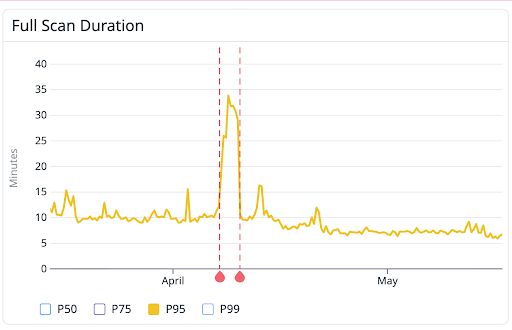 Here we see our 95th percentile of scan times went from 10 minutes, to 7 minutes 30 seconds! 25% faster is pretty good, and matches the data we were seeing.
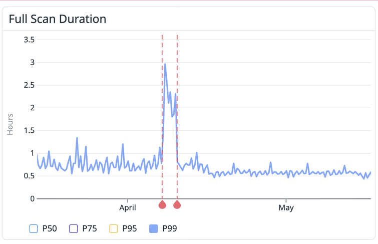 Our P99 went from a very noisy ~45 minutes on average, to a much more consistent 35 minutes.
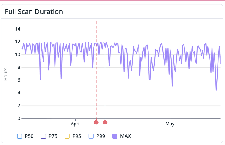 Finally our max scan times are pretty interesting. You can see that before this change, they were closed to pegged at 12 hours. The reason for 12 hours here is that’s our absolute limit for scan times, as after that it becomes increasingly difficult to do things like roll out new changes to our infrastructure. Now our max scan times vary much more, often dipping below 12 for much longer periods of time.
The change to max scan times here and increase in consistency for P99 times are huge for a few reasons. First, the less noisy program durations are, the easier it is for us to set alerts for performance regressions, and reason about future performance improvements. The dip in max times is important as that means the chance of a very large repo scan without additional resources increases significantly, which means it’s a bit easier to onboard users without tweaking as many knobs.
Notably missing here are P50 and P95 times. As mentioned before Semgrep is relatively fast, so for 75% of scans, taint analysis isn’t a huge part of it. Many of our users though have many small repositories that they don’t care much about, and also have a small set of very large repositories (or monorepos), that they do care about. So our P95 is “only” 5% of scans, but of the repositories (and therefore scans) that folks actually care about, it's much, much higher.
For example, here are some traces (so flame graphs representing wall clock time) of two repositories that two of high profile users really care about:


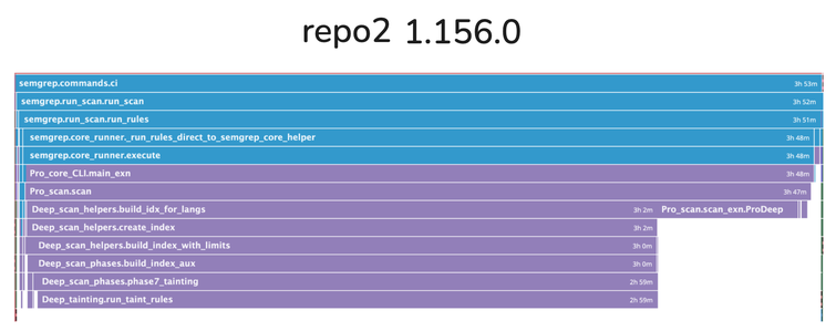
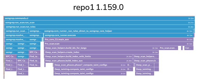
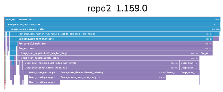 The part labelled "Pro_scan.scan_exn.ProDeep" is where we did taint a second time. "Deep_scan_helpers.create_index" is where we now filter out a ton of work, and do more things in parallel.